How to Practically Diversify Your Investment for Non-financial Analysts (Free Calculator Workbook)
Taking advantage of Portfolio Diversification, the only free lunch in our financial world.
Why Should You Read This?
If you’ve ever wondered whether your investment portfolio is working as hard as you are, this post is for you. By the end, you’ll know how to optimize your portfolio like a pro. Plus, you’ll get a nifty spreadsheet that does the heavy lifting for you. Simply plug in your own investment data, and voilà—instant insights into how to make your money work smarter.
Before we start, if you are not confident with your statistical, mathematical and financial knowledge. Don’t fear. A lot of times, the terminologies sound sophisticated and somewhat intelligent, but really the underlying concept is pretty simple. You will have some experience with Excel, and if you can run (not write) some python code, it will make things easier as well.
Important Notice Content is for informational purposes only and not meant as a recommendation for investment decisions.
Here are some results from my sample analysis.
Download the File and Follow Along
Here’s your toolkit: a downloadable spreadsheet and some step-by-step instructions. Screenshots included to guide you through the process. It’s like having a financial coach on your screen, minus the judgmental glances.
Attachment:Portfolio_diversification.xlsx
To outline the post
Part 1: How to use the calculator
Part 2: How to measure portfolio performance
Part 3: How to optimise it
Part 1: How to use the calculator
I believe the following screenshot should explain how it works probably better than me.
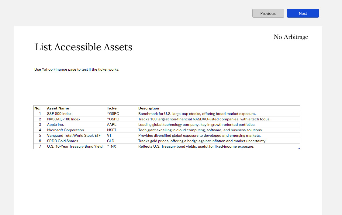
Step #0: List your assets.
Choose Equity or equity like Asset to run this analysis.
You can run this on any assets in theory, such as ETF funds. Fixed income securities (such as corporate bond) should be proceeded with caution, because the price information you are going to collect may not reflect the true return, as part of the return may come from coupon. If the asset doesn’t pay coupon or the asset is a fund that will just re-invest the proceed from the underlying fixe income holdings, that’s fine, as long as the price information reflect the asset return.
You can run this analysis with real estate property assets. you can populate the price index of your local market if there is such available. For periods you don’t have data, you can just use the last period, assuming there is no change. This behaviour in theory underestimates the asset volatility. But in practice, it may not be a bad thing to evaluate asset less often. It is a bit hassle to do because you have to make sure the date column are matched.
Fixed Income Portfolio Optimisation
Fixed Income portfolio typically have their own optimisation framework, such as immunisation. That’s a pretty different objective from Mean-Variance Optimisation framework.
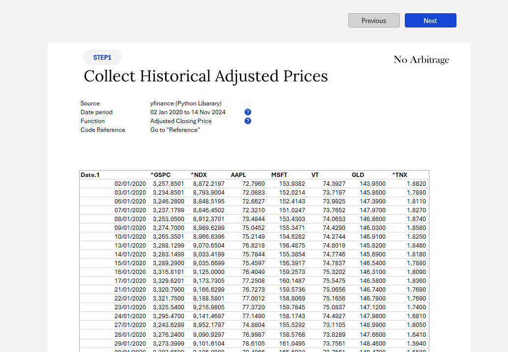
Step #1: Collect adjusted daily price data
In order collect the adjusted price data, you will need to either manually download the data directly from Yahoo Finance or your custom sources. Alternatively, you can use the python scripts below. All you need to do is to replace the line 4
tickers = ["^GSPC", "^NDX", "AAPL", "MSFT", "VT", "GLD", "TSLA"]
in the square brackets, replace these tickers with your own and make sure each is wrapped in either double or single quotation. And then throw this code into runtime,
python code is here
import yfinance as yf
import pandas as pd
import os
tickers = ["^GSPC", "^NDX", "AAPL", "MSFT", "VT", "GLD", "TSLA"]
download_path = '~/Downloads/'
filename = 'yfinance-downloads.csv'
start_date = "2020-01-01"
end_date = "2023-11-14"
# Dictionary to store data
data = {}
# Fetch historical data for each ticker
for ticker in tickers:
    stock_data = yf.download(ticker, start=start_date, end=end_date)
 # Ensure we're using adjusted close prices
    stock_data['Adjusted Price'] = stock_data['Adj Close']
    data[ticker] = stock_data
    print(f"Downloaded data for {ticker} with adjusted prices")
adj_data = {}
for key, value in data.items():
    adj_data[key] = value['Adjusted Price']
df = pd.DataFrame( adj_data )
filepath = os.path.join( download_path,filename )
df.to_csv(filepath)
Step #2: Compute daily return
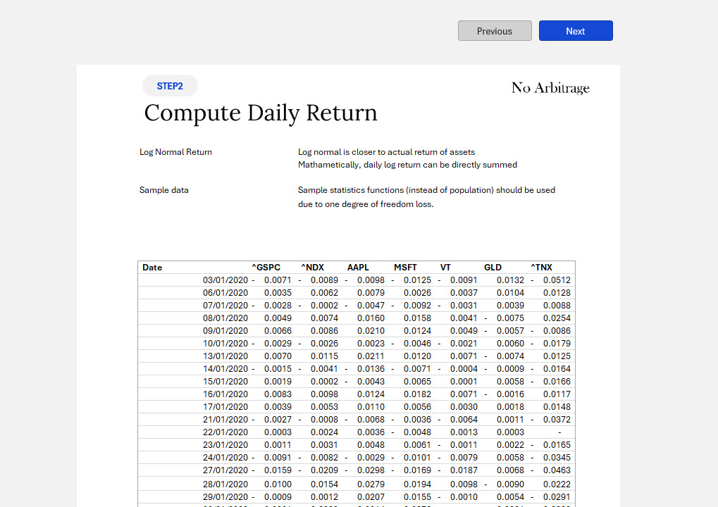
It is worth to mention that when I downloaded the data into the csv file, the data somehow was formatted as text therefore causing problems in subsequent calculation, it may not happen to you. But to show you how I work around it. I save the data from the download csv directly to the worksheet ‘yfinance-downloads’, and I used power query to help me reformat the data.
If you would like to use my method, you can copy past the csv data to replace the existing data in the ‘yfinance-downloads’ page, and then, go to Data tab and click Refresh All bottom under Queries and connection section.
PowerQuery code is here ( in case you are interested). I’ve wrote my own code to make this query dynamic, able to process your custom data, most likely with different table headings (asset tickers) from mine.
let
    Source = Excel.CurrentWorkbook(){[Name="Table2"]}[Content],
    Splitbydelimiter = Table.SplitColumn(Source, "Date", Splitter.SplitTextByEachDelimiter({" "}, QuoteStyle.Csv, false), {"Date.1", "Date.2"}),
    withDates = Table.RemoveColumns(Splitbydelimiter,{"Date.2"}),

    withoutDates = Table.RemoveColumns(withDates,{"Date.1"}),
    columnheader = Table.ColumnNames(withoutDates),
    transform = List.Transform( columnheader, each {_, type number} ),

    TypeChange = Table.TransformColumnTypes(withDates,transform),
    TypeChange2 = Table.TransformColumnTypes(TypeChange,  {{"Date.1",type date}})
in
    TypeChange2
Step #3 : Using Solver to get the allocation.
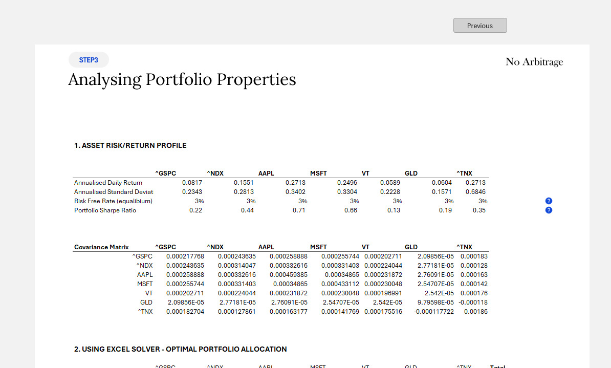
Please find instructions in Part 3.
Part 2 can be more interesting to read for people with certain level of financial knowledge or people come from a mathematical, computer science or engineering background, it is perfectly okay if you want to skip these. It mainly explains the certain choices of approach in the worksheet, such one specific return calculation is used instead of another.
Part 2: How to measure portfolio performance
Intuitively, we are looking for a system to describe the risks and return properties of a portfolio. One of such system is Mean Variance Analysis.
Here’s where the magic happens—optimizing your portfolio using some fancy math.
Mean-Variance Optimization
Applying this framework, we formalise the portfolio performances in the following three measures. We use
- Expected return to describe returns
- Portfolio Variance (or standard deviation) to describe risks
- Shape Ratio to measure the risk/return trade-off efficiency. It measures how much return you generate for every unit of risk taken.
That’s it. Job’s done! Simple right? Now because you asked, I am going to dive a little deeper, only for those there are interested.
The standard mathematical formula is provided alongside the matrix algebra version, which is very elegant and efficient for its brevity.
See the math formulas
| Portfolio Statistics | Standard Math | Matrix Algebra | Additional Notes |
|---|---|---|---|
| Expected Return |
|
|
Return calculation typically is In standard form However, log normal form is much more popular. |
| Portfolio Variance | in Covariance terms In correlation terms Example with two assets} |
|
|
| Sharpe Ratio |
|
|
Discussion #1: Why use Log return instead of standard return formula?
- Additive . the mathematically property of log provides us the ability to link period return by summing them instead of using geographic linking.
- Asset return is not normally distributed. It typically has a fat left tail and think right tail in real world
- This form is also widely used in derivative market where interest rate compounding period is assumed to be infinite. and you have $ P_0 \cdot e^{E(R)T} = P_1 $
Discussion #2: Daily Adjusted Closing Price
We used Daily Adjusted Closing Price to calculate returns. Adjustments are carried out to account for stock split, dividends and new issuance.
Do you need to adjust for inflation? Not necessary. As long as all your prices are consistent and results will also remain consistent.
Do we need to adjust for FX if I have a multi-currency portfolio? Not necessary. This topic is worth a few posts to explain. For simplicity, because the returns are in percentage turns, as long as the weighting is applied after converting asset values into a common currency, the results will be valid.
Discussion #3: Over what period should I run analysis for (Horizon)
In common sense, the backward-looking historical period should be in line with your forward-looking investment horizon. Statistically, a full business cycle period is likely provide more informative and less biased prediction.
In our file, a roughly four-year period is used. In order to better predict future returns, select a period that is stationary, ideally cover a business cycle, despite not being essential.
This data is provided by Yahoo Finance (through yfinance python module, source code already provided in the file).
Discussion #4: Portfolio Variance
This measure captures the variation of returns. This measure has many flaws.
- First, Two portfolios with very different return distributions can have similar variances. Only if the return distribution is Normal, then, you can define a unique distribution with Mean and Variance. It is widely observed that asset returns are not perfectly normal.
- Second, only downward variations in price are considered risks by investors, positive variations in price are not perceived as risks. VaR (Value at Risk) capture only the downside variations therefore can potentially serve as a better alternative. (VaR falls out of the scope of this post.)
Discussion #5: Covariance Matrix
Example of Covariance Matrix
\Sigma =
\begin{bmatrix}
\sigma_{1}^2 & \sigma_{12} & \sigma_{13}
\sigma_{12} & \sigma_{2}^2 & \sigma_{23}
\sigma_{13} & \sigma_{23} & \sigma_{3}^2
\end{bmatrix}
\
Variance is defined as $V(x)=\frac{1}{N-1}\Sigma(x_i-μ)^2$ Covariance between two random variables x and y (or columns of a matrix) is defined as $Cov(x,y)= \frac{1}{N-1} \Sigma (x_i−μ_x)(y_i−μ_y) $ and $Cov(x,x)=V(x)$
The term covariance matrix may be misleading to you. It is not any sort of a special matrix. It is simply set of variances and covariances between pairs of columns. A position of any element in the covariance matrix corresponds to variance/covariance between a pair of two columns, e.g. a number located in 3rd row and 2nd column in the covariance matrix represents covariance between 3rd and 2nd columns of matrix A. $Cov(x,y)=Cov(y,x)$ , therefore covariance matrix is symmetric.
- For N asset portfolio, you will have N x N covariance matrix.
- Any covariance matrix is symmetric and positive semi-definite and its main diagonal contains variances.
- Covariance matrix can only be calculated through actual underlying price data. Practically, the most used two ways to generate covariance matrix in Excel are
- use Data Analysis Toolpak (Add-In) to calculate the covariance.
- use Excel scripting formula
In the template file, I used the Excel scripting formula to calculate the covariance matrix. This allows dynamic evaluation (Analysis Toolpak require manual re-do the analysis when you change data) and it also avoids Add-in compatibility issues.
- This is the fundamental piece of portfolio theory. the covariance matrix captures the potential of diversification among component assets.
- Diversification is arguably the only free lunch in the financial world.
Discussion #6: Weighting
We assume you won’t go full “Wolf of Wall Street” by short-selling. All weights in your portfolio will stay positive. Plus, you’ll invest fully—because letting money sit idle is like letting a treadmill gather dust.
In our template file, we specify that each asset must take at least 5% of the portfolio value. This constraints avoids the situation of short selling. And if one can borrow at risk free rate, the portfolio return/return can be further optimised to investor’s advantage. Under that condition, we can even constructing a market portfolio and customised a risk / return profile to investor’s preference. In the future, I will dedicate a post for this topic.
Discussion #7: Sharp Ratio
The Sharpe Ratio is like a quick fitness test for your portfolio: How much return are you getting for every unit of risk? Are you taking risks efficiently?
The Efficient Frontier is where your portfolio hits the sweet spot—maximizing returns for a given level of risk.
Sharp ratio provides a universal, straightforward and useful concept to compare investment performance based on mean and variance. We subtract a risk-free rate from the portfolio return to separate the riskless and risky portion of returns. Then we compare the return premium to the added risk.
We will discuss efficient frontier in a separate post.
Markowitz demonstrated that diversification reduces risk so that investors can earn the same return with lower risk, or a higher return for the same risk. He argued that “diversification is the only free lunch in finance.” Investors were urged to diversify across stocks, countries and asset classes.
Teamwork Makes the Dream Work Think of this as figuring out which assets in your portfolio get along and which are the drama queens. Assets with low or negative covariance balance each other out, reducing your overall risk. If many of assets share similar temper, may god bless you.
Section Summary
So based on what we discussed above, the next step should be intuitive, we want to maximise the return and minimise the risks based on the portfolio.
Next, we can leverage the Excel Solver tool to do the leg work and compute an optimal results.
-
We are standing on Giants shoulder
Economist Harry Markowitz introduced MPT in a 1952 essay for which he was later awarded a Nobel Memorial Prize in Economic Sciences (Markowitz model).
This Mean Variance Optimisation framework is a big thing in Finance and is often mixed with a more significant term, [Modern portfolio theory](https://en.wikipedia.org/wiki/Modern_portfolio_theory). (like all significant and difficult-to-understand things in our life, it has an acronym, MPT).
Part 3: Solving the Optimisation Problem
This is very simple,
1. Switching on Solver feature in Excel if it is not on yet.
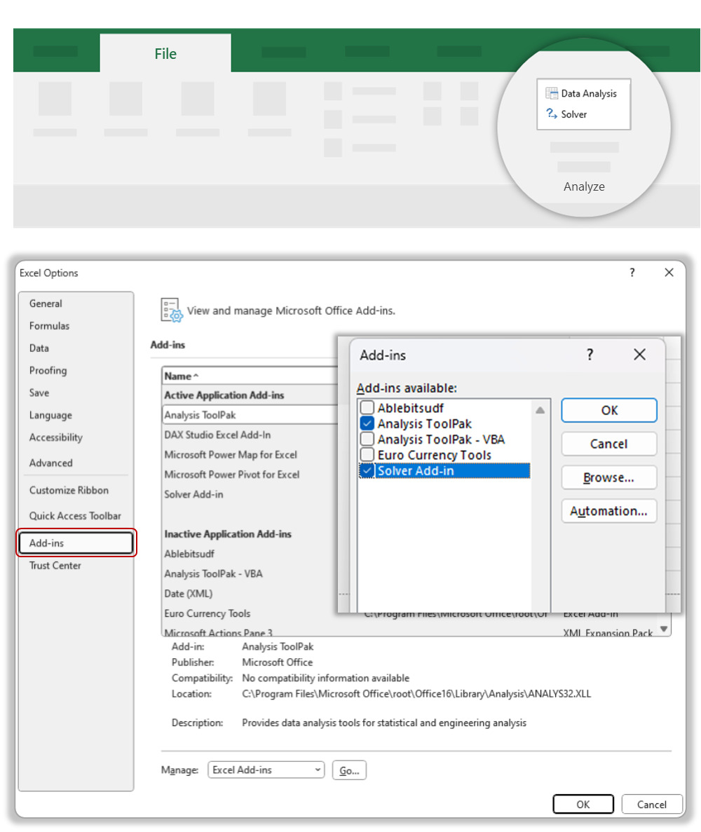
2. Once enabled, you can find them here
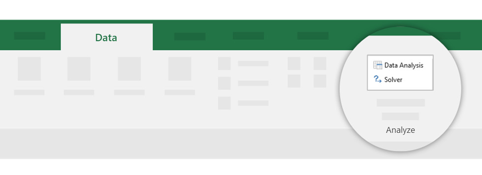
Then, go straight to the point!
3. Configurations Guide
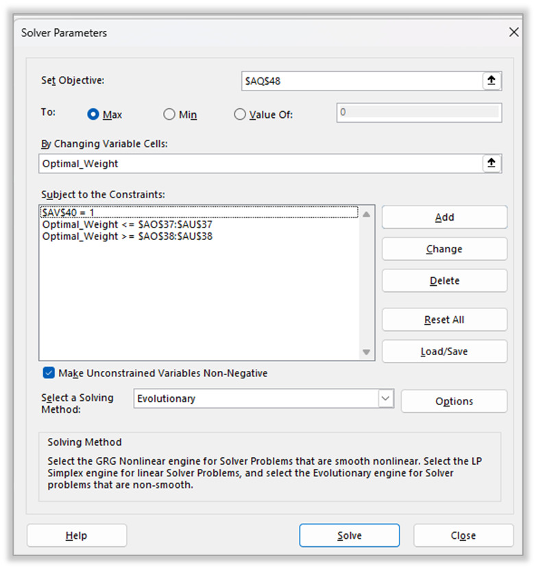
- Objective: Set this to be the shape ratio, set max as a goal.
- Changing variables: Select the portfolio weighting array
- Constraints: based on traditional insights to have set some guideline limits for each portfolio asset, for example, no asset should have a weight that’s 10x time than the smallest asset in the portfolio.
- Solving method
Comparing Simplex, GRG Non-Linear and Evolution method in Excel Solver.
Closing Note
This post is meant to be a practical one. A lot of ideas came up while editing this post. I will dedicate posts for some of the topics below
- Fixed Income portfolio optimisation.
- Market Portfolio
- From Portfolio Theory to CAPM Model and M-M theory
- Optimisation - Basic Operational Research